Harnessing symmetry to find the center of a diffraction pattern

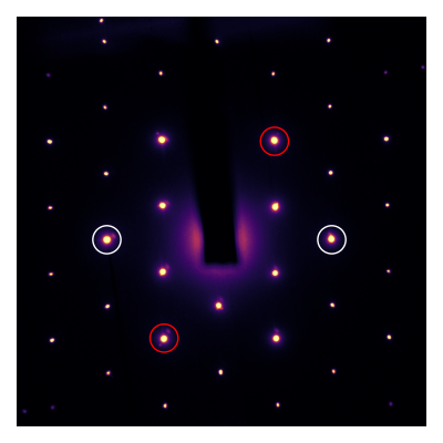
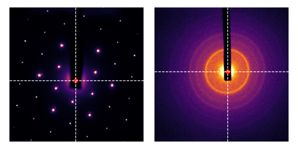
Ultrafast electron diffraction involves the analysis of diffraction patterns. Here is an example diffraction pattern for a thin (<100nm) flake of graphite¹:

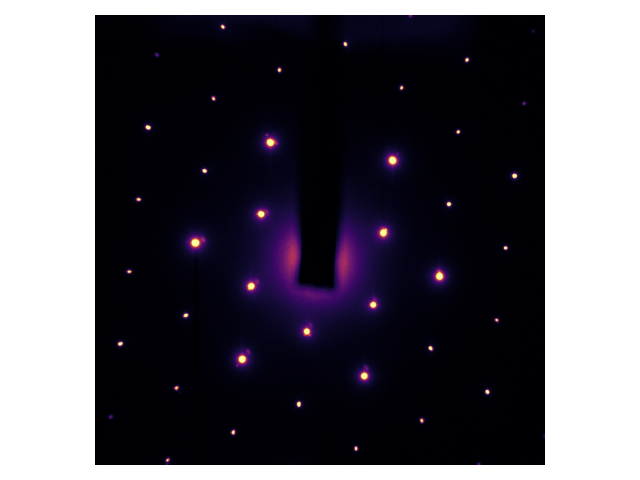
A diffraction pattern is effectively the intensity of the Fourier transform. Given that crystals like graphite are well-ordered, the diffraction peaks (i.e. Fourier components) are very large. You can see that the diffraction pattern is six-fold symmetric; that’s because the atoms in graphite arrange themselves in a honeycomb pattern, which is also six-fold symmetric. In these experiments, the fundamental Fourier component is so strong that we need to block it. That’s what that black beam-block is about.

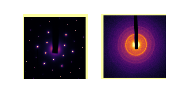
There are crystals that are not as well-ordered as graphite. Think of a powder made of many small crystallites, each being about 50nm x 50nm x 50nm. Diffraction electrons through a sample like that results in a kind of average of all possible diffraction patterns. Here’s an example with polycrystalline Chromium:

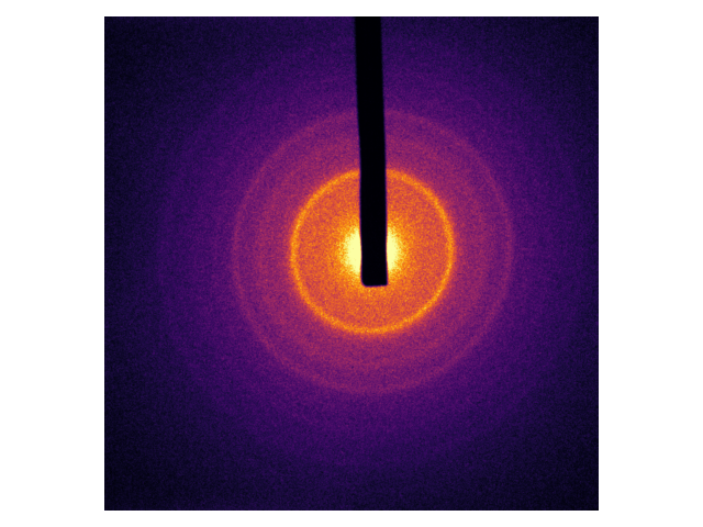
Each ring in the above pattern pattern corresponds to a Fourier component. Notice again how symmetric the pattern is; the material itself is symmetric enough that the fundamental Fourier component needs to be blocked.

For my work on iris-ued, a data analysis package for ultrafast electron scattering, I needed to find a reliable, automatic way to get the center of such diffraction patterns to get rid of the manual work required now. So let’s see how!

First try: center of mass

A first naive attempt might start with the center-of-mass, i.e. the average of pixel positions weighted by their intensity. Since intensity is symmetric about the center, the center-of-mass should coincide with the actual physical center of the image.

Good news, scipy’s ndimage module exports such a function: center_of_mass. Let’s try it:

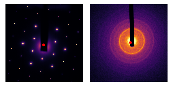
Not bad! Especially in the first image, really not a bad first try. But I’m looking for something pixel-perfect. Intuitively, the beam-block in each image should mess with the calculation of the center of mass. Let’s define the following areas that we would like to ignore:

Masks are generally defined as boolean arrays with True (or 1) where pixels are valid, and False (or 0) where pixels are invalid. Therefore, we should ignore the weight of masked pixels. scipy.ndimage.center_of_mass does not support this feature; we need an extension of center_of_mass:

def center_of_mass_masked(im, mask):
    rr, cc = np.indices(im.shape)
    weights = im * mask.astype(im.dtype)

    r = np.average(rr, weights=weights)
    c = np.average(cc, weights=weights)
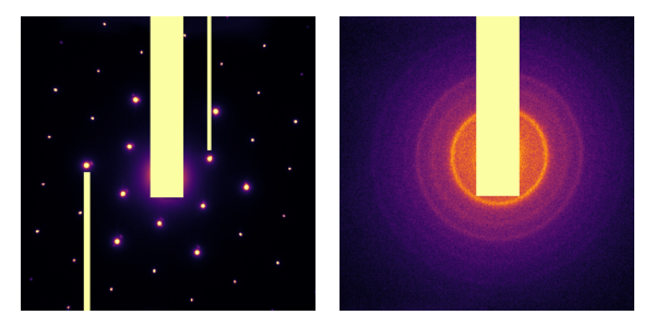
    return r, c

This is effectively an average of the row and column coordinates (rr and cc) weighted by the image intensity. The trick here is that mask.astype(im.dtype) is 0 where pixels are “invalid”; therefore they don’t count in the average! Let’s look at the result:

I’m not sure if it’s looking better, honestly. But at least we have an approximate center! That’s a good starting point that feeds in to the next step.

Friedel pairs and radial inversion symmetry

In his thesis², which is now also a book, Nelson Liu describes how he does it:

A rough estimate of its position is obtained by calculating the ‘centre of intensity’ or intensity-weighted arithmetic mean of the position of > 100 random points uniformly distributed over the masked image; this is used to match diffraction spots into Friedel pairs amongst those found earlier. By averaging the midpoint of the lines connecting these pairs of points, a more accurate position of the centre is obtained.

Friedel pairs are peaks related by inversion through the center of the diffraction pattern. The existence of these pairs is guaranteed by crystal symmetry. For polycrystalline patterns, Friedel pairs are averaged into rings; rings are always inversion-symmetric about their centers. Here’s an example of two Friedel pairs:

The algorithm by Liu was meant for single-crystal diffraction patterns with well-defined peaks, and not so much for rings. However, we can distill Liu’s idea into a new, more general approach. If the approximate center coincides with the actual center of the image, then the image should be invariant under radial-inversion with respect to the approximate center. Said another way: if the image $I$ is defined on polar coordinates $(r, \theta)$, then the center maximizes correlation between $I(r, \theta)$ and $I(-r, \theta)$. Thankfully, computing the masked correlation between images is something I’ve worked on before!

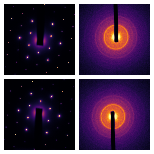
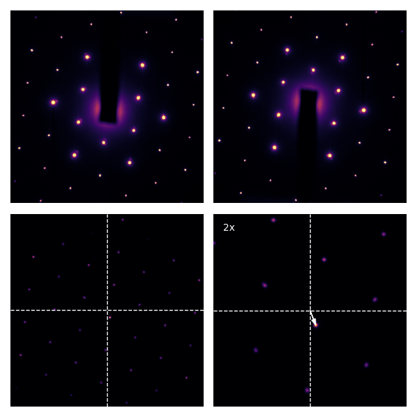
Let’s look at what radial inversion looks like. There are ways to do it with interpolation, e.g. scikit-image’s warp function. However, in my testing, this is incredibly slow compared to what I will show you. A faster approach is to consider that if the image was centered on the array, then radial inversion is really flipping the direction of the array axes; that is, if the image array I has size (128, 128), and the center is at (64, 64), the radial inverse of I is I[::-1, ::-1] (numpy) / flip(flip(I, 1), 2) (MATLAB) / I[end:-1:1,end:-1:1] (Julia). Another important note is that if the approximate center of the image is far from the center of the array, the overlap between the image and its radial inverse is limited. Consider this:

If we cropped out the bright areas around the frame, then the approximate center found would coincide with the center of the array; then, radial inversion is very fast.

Now, especially for the right column of images, it’s pretty clear that the approximate center wasn’t perfect. The correction to the approximate center is can be calculated with the masked normalized cross-correlation^{3 4}:

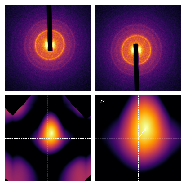
The cross-correlation in the bottom right corner (zoomed by 2x) shows that the true center is the approximate center we found earlier, corrected by the small shift (white arrow)! For single-crystal diffraction patterns, the resulting is even more striking:

We can put the two steps together and determine a pixel-perfect center:

Bonus: low-quality diffraction

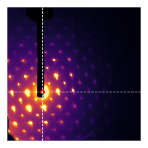
Here’s a fun consequence: the technique works also for diffraction patterns that are pretty crappy and very far off center, provided that the asymmetry in the background is taken care-of:

Conclusion

In this post, we have determined a robust way to compute the center of a diffraction pattern without any parameters, by making use of a strong invariant: radial inversion symmetry. My favourite part: this method admits no free parameters!

If you want to make use of this, take a look at autocenter, a new function that has been added to scikit-ued.