Efficient rolling statistics

In the context of an array, rolling operations are operations on a set of values which are computed at each index of the array based on a subset of values in the array. A common rolling operation is the rolling mean, also known as the moving average.

The best way to understand is to see it in action. Consider the following list:

[0, 1, 2, 3, 4, 3, 2, 1]

The rolling average with a window size of 2 is:

[ (0 + 0)/2, (0 + 1)/2, (1 + 2)/2, (2 + 3)/2, (3 + 4)/2, (4 + 3)/2, (3 + 2)/2, (2 + 1)/2]

or

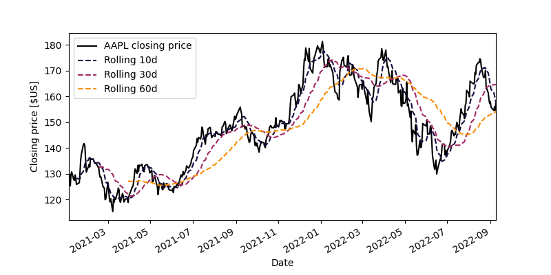
[0, 0.5, 1.5, 2.5, 3.5, 3.5, 2.5, 1.5]

Rolling operations such as the rolling mean tremendously useful at my work. When working with time-series, for example, the rolling mean may be a good indicator to include as part of machine learning feature engineering or trading strategy design. Here’s an example of using the rolling average price of AAPL stock as an indicator:

The problem is that rolling operations can be rather slow if implemented improperly. In this post, I’ll show you how to implement efficient rolling statistics using a method based on recurrence relations.

In principle, a general rolling function for lists might have the following type signature:

rolling :: Int        -- ^ Window length
        -> ([a] -> b) -- ^ Rolling function, e.g. the mean or the standard deviation
        -> [a]        -- ^ An input list of values
        -> [b]        -- ^ An output list of values

In this hypothetical scenario, the rolling function of type [a] -> b receives a sublist of length $M$, the window length. The problem is, if the input list has size $N$, and the window has length $M$, the complexity of this operation is at best $\mathcal{O}(N \cdot M)$. Even if you’re using a data structure which is more efficient than a list – an array, for example –, this is still inefficient.

Let’s see how to make this operation $\mathcal{O}(N)$, i.e. constant in the window length!

Recurrence relations and the rolling average

The recipe for these algorithms involves constructing the recurrence relation of the operation. A recurrence relation is a way to describe a series by expressing how a term at index $i$ is related to the term at index $i-1$.

Let proceed by example. Consider a series of values $X$ like so:

$$X = \left[ x_0, x_1, ...\right]$$

We want to calculate the rolling average $\bar{X} = \left[ \bar{x}_0, \bar{x}_1, ... \right]$ of series $X$ with a window length $N$. The equation for the $j$^th term, $\bar{x}_j$ is given by:

$$\bar{x}_j = \frac{1}{N}\sum_{i=j - N + 1}^{N} x_i = \frac{1}{N} \sum \left[ x_{j - N + 1}, x_{j - N + 2}, ..., x_{j} \right]$$

Now let’s look at the equation for the $(j-1)$^th term:

$$\bar{x}_{j-1} = \frac{1}{N}\sum_{i=j - N}^{j-1} x_i = \frac{1}{N} \sum \left[ x_{j - N}, x_{j - N + 1}, ..., x_{j-1} \right]$$

Note the large overlap between the computation of $\bar{x}_j$ and $\bar{x}_{j-1}$; in both cases, you need to sum up $\left[ x_{j-N+1}, x_{j-N+2}, ..., x_{j-1} \right]$

Given that the overlap is very large, let’s take the difference between two consecutive terms, $\bar{x}_j$ and $\bar{x}_{j-1}$:

$$\begin{aligned} \bar{x}_j - \bar{x}_{j-1} &= \frac{1}{N} \sum \left[ x_{j - N + 1}, x_{j - N + 2}, ..., x_j \right] - \frac{1}{N} \sum \left[ x_{j - N}, x_{j - N + 1}, ..., x_{j-1} \right] \\ &= \frac{1}{N} \sum \left[ -x_{j-N} + x_{j - N + 1} - x_{j - N + 1} + x_{j - N + 2} - x_{j - N + 2} + ... + x_{j-1} - x_{j-1} + x_j\right] \\ &= \frac{1}{N} ( x_{j} - x_{j - N} ) \end{aligned}$$

Rewriting a little:

$$\bar{x}_j = \bar{x}_{j-1} + \frac{1}{N} ( x_j - x_{j-N} )$$

This is the recurrence relation of the rolling average with a window of length $N$. It tells us that for every term of the rolling average series $\bar{X}$, we only need to involve two terms of the original series $X$, regardless of the window. Awesome!

Haskell implementation

Let’s implement this in Haskell. We’ll use the vector library which is much faster than lists for numerical calculations like this, and comes with some combinators which make it pretty easy to implement the rolling mean. Regular users of vector will notice that the recurrence relation above fits the scanl use-case. If you’re unfamiliar, scanl is a function which looks like this:

scanl :: (b -> a -> b) -- ^ Combination function
      -> b             -- ^ Starting value
      -> Vector a      -- ^ Input
      -> Vector b      -- ^ Output

For example:

>>> import Data.Vector as Vector
>>> Vector.scanl (+) 0 (Vector.fromList [1, 4, 7, 10])
[1, 5, 12, 22]

If we decompose the example:

[    0 + 1                 -- 1
,   (0 + 1) + 4            -- 5
,  ((0 + 1) + 4) + 7       -- 12
, (((0 + 1) + 4) + 7) + 10 -- 22
]

In this specific case, Vector.scanl (+) 0 is the same as numpy.cumsum if you’re more familiar with Python. In general, scanl is an accumulation from left to right, where the “scanned” term at index i depends on the value of the input at indices i and the scanned term at i-1. This is perfect to represent recurrence relations. Note that in the case of the rolling mean recurrence relation, we’ll need access to the value at index i and i - N, where again N is the length of the window. The canonical way to operate on more than one array at once elementwise is the zip* family of functions.

-- from the `vector` library
import           Data.Vector ( Vector )   
import qualified Data.Vector as Vector

-- | Perform the rolling mean calculation on a vector.
rollingMean :: Int            -- ^ Window length
            -> Vector Double  -- ^ Input series
            -> Vector Double  
rollingMean window vs
    = let w     = fromIntegral window 
          -- Starting point is the mean of the first complete window
          start = Vector.sum (Vector.take window vs) / w
          
          -- Consider the recurrence relation mean[i] = mean[i-1] + (edge - lag)/w 
          -- where w    = window length
          --       edge = vs[i]
          --       lag  = vs[i - w]
          edge = Vector.drop window vs
          lag  = Vector.take (Vector.length vs - window) vs

        -- mean[i] = mean[i-1] + diff, where diff is:
          diff = Vector.zipWith (\p n -> (p - n)/w) edge lag
      
    -- The rolling mean for the elements at indices i < window is set to 0
       in Vector.replicate (window - 1) 0 <> Vector.scanl (+) start diff

With this function, we can compute the rolling mean like so:

>>> import Data.Vector as Vector
>>> rollingMean 2 $ Vector.fromList [0,1,2,3,4,5]
[0.0,1.5,2.5,3.5,4.5]

Complexity analysis

Let’s say the window length is $N$ and the input array length is $n$. The naive algorithm has complexity $\mathcal{O}(n \cdot N)$. On the other hand, rollingMean has a complexity of $\mathcal{O}(n + N)$:

• Vector.sum to compute start is $\mathcal{O}(N)$;
• Vector.replicate (window - 1) has order $\mathcal{O}(N)$
• Vector.drop and Vector.take are both $\mathcal{O}(1)$;
• Vector.scanl and Vector.zipWith are both $\mathcal{O}(n)$ (and in practice, these operations should get fused to a single pass);

However, usually $N << n$. For example, at work, we typically roll 10+ years of data with a window on the order of days / weeks. Therefore, we have that rollingMean scales linearly with the length of the input ($\mathcal{O}(n)$)

Efficient rolling variance

Now that we’ve developed a procedure on how to determine an efficient rolling algorithm, let’s do it for the (unbiased) variance.

Again, consider a series of values:

$$X = \left[ x_0, x_1, ...\right]$$

We want to calculate the rolling variance $\sigma^2(X)$ of series $X$ with a window length $N$. The equation for the $j$^th term, $\sigma^2_j$ is given by:

$$\sigma^2_j = \frac{1}{N - 1}\sum_{i=j - N + 1}^{j} (x_i - \bar{x}_j)^2 = \frac{1}{N-1} \sum \left[ (x_{j - N + 1} - \bar{x}_j)^2, ..., (x_j - \bar{x}_j)^2 \right]$$

where $\bar{x}_i$ is the rolling mean at index $i$, just like in the previous section. Let’s simplify a bit by expanding the squares:

$$\begin{aligned} (N - 1) ~ \sigma^2_j &= \sum_{i=j-N+1}^{j} (x_i - \bar{x}_j)^2 \\ &= N\bar{x}^2_j + \sum_{i=j - N + 1}^{j} x^2_i - 2 x_i \bar{x}_j \end{aligned}$$

We note here that $\sum_{i=j - N + 1}^{j} x_i \equiv N \bar{x}_j$, which allows to simplify the equation further:

$$\begin{aligned} (N - 1) ~ \sigma^2_j &= N\bar{x}^2_j - 2 N \bar{x}^2_j + \sum_{i=j - N + 1}^{j} x^2_i \\ &= -N\bar{x}^2_j + \sum_{i=j - N + 1}^{j} x^2_i \end{aligned}$$

This leads to the following difference between consecutive rolling unbiased variance terms:

$$\begin{aligned} (N - 1) \left( \sigma^2_j - \sigma^2_{j-1} \right) &= N\bar{x}^2_{j - 1} - N\bar{x}^2_j + \sum_{i=j - N + 1}^{j} x^2_i - \sum_{i'=j - N}^{j-1} x^2_{i'} \\ &= N\bar{x}^2_{j - 1} - N\bar{x}^2_j + x^2_j - x^2_{j-N} \end{aligned}$$

and therefore, the recurrence relation:

$$\sigma^2_j = \sigma^2_{j-1} + \frac{1}{N-1} \left[ N\bar{x}^2_{j - 1} - N\bar{x}^2_j + x^2_j - x^2_{j - N} \right]$$

This recurrence relation looks pretty similar to the rolling mean recurrence relation, with the added wrinkle that you need to know the rolling mean in advance.

Haskell implementation

Let’s implement this in Haskell again. We can re-use our rollingMean. We’ll also need to compute the unbiased variance in the starting window; I’ll use the statistics library for brevity, but it’s easy to implement yourself if you care about minimizing dependencies.

-- from the `vector` library
import           Data.Vector ( Vector )   
import qualified Data.Vector as Vector
-- from the `statistics` library
import           Statistics.Sample ( varianceUnbiased )

rollingMean :: Int          
            -> Vector Double
            -> Vector Double
rollingMean = (...)  -- see above

-- | Perform the rolling unbiased variance calculation on a vector.
rollingVar :: Int          
           -> Vector Double
           -> Vector Double
rollingVar window vs
    = let start   = varianceUnbiased $ Vector.take window vs
          n       = fromIntegral window
          ms      = rollingMean window vs
        
          -- Rolling mean terms leading by N
          ms_edge = Vector.drop window ms
          -- Rolling mean terms leading by N - 1
          ms_lag  = Vector.drop (window - 1) ms
          
          -- Values leading by N
          xs_edge = Vector.drop window vs
          -- Values leading by 0
          xs_lag  = vs
          
          -- Implementation of the recurrence relation, minus the previous term in the series
          -- There's no way to make the following look nice, sorry.
          -- N * \bar{x}^2_{N-1} - N * \bar{x}^2_{N} + x^2_N - x^2_0
          term xbar_nm1 xbar_n x_n x_0 = (n * (xbar_nm1**2) - n * (xbar_n ** 2) + x_n**2 - x_0**2)/(n - 1)
        
    -- The rolling variance for the elements at indices i < window is set to 0
       in Vector.replicate (window - 1) 0 <> Vector.scanl (+) start (Vector.zipWith4 term ms_lag ms_edge xs_edge xs_lag)

Note that it may be benificial to reformulate the $N\bar{x}^2_{j - 1} - N\bar{x}^2_j + x^2_j - x^2_{j - N}$ part of the recurrence relation to optimize the rollingVar function. For example, is it faster to minimize the number of exponentiations, or multiplications? I do not know, and leave further optimizations aside.

Complexity analysis

Again, let’s say the window length is $N$ and the input array length is $n$. The naive algorithm still has complexity $\mathcal{O}(n \cdot N)$. On the other hand, rollingVar has a complexity of $\mathcal{O}(n + N)$:

• varianceUnbiased to compute start is $\mathcal{O}(N)$;
• Vector.replicate (window - 1) has order $\mathcal{O}(N)$
• Vector.drop and Vector.take are both $\mathcal{O}(1)$;
• Vector.scanl and Vector.zipWith4 are both $\mathcal{O}(n)$ (and in practice, these operations should get fused to a single pass);

Since usually $N << n$, as before, we have that rollingVar scales linearly with the length of the input ($\mathcal{O}(n)$).

Bonus: rolling Sharpe ratio

The Sharpe ratio¹ is a common financial indicator of return on risk. Its definition is simple. Consider excess returns in a set $X$. The Sharpe ratio $S(X)$ of these excess returns is:

$$S(X) = \frac{\bar{X}}{\sigma_X}$$

For ordered excess returns $X = \left[ x_0, x_1, ... \right]$, the rolling Sharpe ratio at index $j$ is:

$$S_j = \frac{\bar{x}_j}{\sigma_j}$$

where $\bar{x}_j$ and $\sigma_j$ are the rolling mean and standard deviation at index $j$, respectively.

Since the rolling variance requires knowledge of the rolling mean, we can easily compute the rolling Sharpe ratio by modifying the implementation of rollingVariance:

-- from the `vector` library
import           Data.Vector ( Vector )   
import qualified Data.Vector as Vector
-- from the `statistics` library
import           Statistics.Sample ( varianceUnbiased )

rollingMean :: Int          
            -> Vector Double
            -> Vector Double
rollingMean = (...)  -- see above

rollingSharpe :: Int          
              -> Vector Double
              -> Vector Double
rollingSharpe window vs
    = let start   = varianceUnbiased $ Vector.take window vs
          n       = fromIntegral window
          ms      = rollingMean window vs
          
          -- The following expressions are taken from rollingVar
          ms_edge = Vector.drop window ms
          ms_lag  = Vector.drop (window - 1) ms
          xs_edge = Vector.drop window vs
          xs_lag  = vs
          term xbar_nm1 xbar_n x_n x_0 = (n * (xbar_nm1**2) - n * (xbar_n ** 2) + x_n**2 - x_0**2)/(n - 1)

          -- standard deviation from variance
          std = sqrt <$> Vector.scanl (+) start (Vector.zipWith4 term ms_lag ms_edge xs_edge xs_lag)
        
    -- The rolling Sharpe ratio for the elements at indices i < window is set to 0
       in Vector.replicate (window - 1) 0 <> Vector.zipWith (/) (Vector.drop window ms) std

Conclusion

In this blog post, I’ve shown you a recipe to design rolling statistics algorithms which are efficient (i.e. $\mathcal{O}(n)$) based on recurrence relations. Efficient rolling statistics as implemented in this post are an essential part of backtesting software, which is software to test trading strategies.

All code is available in this Haskell module.