Filtering noise with discrete wavelet transforms

All experimental data contains noise. Distinguishing between measurement and noise is an important component of any data analysis pipeline. However, different noise-filtering techniques are suited to different categories of noise.

In this post, I’ll show you a class of filtering technique, based on discrete wavelet transforms, which is suited to noise that cannot be filtered away with more traditional techniques – such as ones that rely on the Fourier transform. This has been important in my past research^{1 2}, and I hope that this can help you too.

Integral transforms

A large category of filtering techniques are based on integral transforms. Broadly speaking, an integral transform $T$ is an operation that is performed on a function $f$ and builds a function $T\left[ f\right]$ which is defined on a variable $s$, such that:

$$T\left[ f \right](s) = \int dt ~ f(t) \cdot K(t, s)$$

Here, $K$ (for kernel) is a function which “selects” which parts of $f(t)$ are important as a fixed $s$. Note that for an integral transform to be useful as a filter, we’ll need the ability to invert the transformation, i.e. there exists an inverse kernel $K^{-1}(s, t)$ such that:

$$f(t) = \int ds ~ \left( T \left[ f\right] (s) \right) \cdot K^{-1}(s,t)$$

All of this was very abstract, so let’s look at a concrete example: the Fourier transform. The Fourier transform is an integral transform where³:

$$\begin{align} K(t, \omega) &\equiv \frac{e^{-i \omega t}}{\sqrt{2 \pi}}\\ K^{-1}(\omega, t) &\equiv e^{i \omega t}\\ \omega & \in \mathbb{R} \end{align}$$

There are many other integral transforms, such as:

• The Laplace transform ($K(t, s) \equiv e^{- s t}$) which is useful to solve linear ordinary differential equations;
• The Legendre transforms ($K_n(t, s) \equiv P_n(s)$, where $P_n$ is the n^th Legendre polynomial) which is used to solve for electron motion in hydrogen atoms;
• The Radon transform (for which I cannot write down a kernel) which is used to analyze computed tomography data.

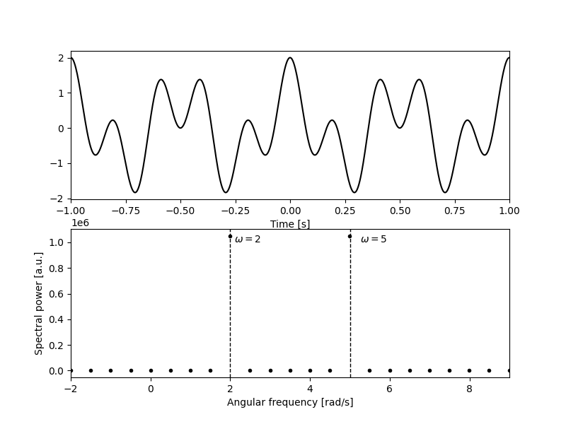
So why are integral transforms interesting? Well, depending on the function $f(t)$ you want to transform, you might end up with a representation of $f$ in the transformed space, $T \left[ f\right] (s)$, which has nice properties! Re-using the Fourier transform for a simple, consider a function made up of two well-defined frequencies:

$$f(t) \equiv e^{-i ~ 2t} + e^{-i ~ 5t}$$

The representation of $f(t)$ in frequency space – the Fourier transform of $f$, $F\left[ f\right](\omega)$ – is very simple:

$$F\left[ f\right](\omega) = \sqrt{2 \pi} \left[ \delta(\omega - 2) + \delta(\omega - 5) \right]$$

The Fourier transform of $f$ is perfectly localized in frequency space, being zero everywhere except at $\omega=2$ and $\omega=5$. Functions composed of infinite waves (like the example above) always have the nice property of being localized in frequency space, which makes it easy to manipulate them… like filtering some of their components away!

Discretization

It is much more efficient to use discretized versions of integral transforms on computers. Loosely speaking, given a discrete signal composed of $N$ terms $x_0$, …, $x_{N-1}$:

$$T\left[ f \right](k) = \sum_n x_n \cdot K(n, k)$$

i.e. the integral is now a finite sum. For example, the discrete Fourier transform of the signal $x_n$, $X_k$, can be written as:

$$X_k = \sum_n x_n \cdot e^{-i 2 \pi k n / N}$$

and its inverse becomes:

$$x_n = \frac{1}{N}\sum_k X_k \cdot e^{i 2 \pi k n / N}$$

This is the definition used by numpy, for example. Let’s use this definition to compute the discrete Fourier transform of $f(t) \equiv e^{-i ~ 2t} + e^{-i ~ 5t}$:

Using the discrete Fourier transform to filter noise

Let’s add some noise to our signal and see how we can use the discrete Fourier transform to filter it away. The discrete Fourier transform is most effective if your noise has some nice properties in frequency space. For example, consider high-frequency noise:

$$N(t) = \sum_{\omega=20}^{50} \sin(\omega t + \phi_{\omega})$$

where $\phi_\omega$ are random phases, one for each frequency component of the noise. While the signal looks very noisy, it’s very obvious in frequency-space what is noise and what is signal:

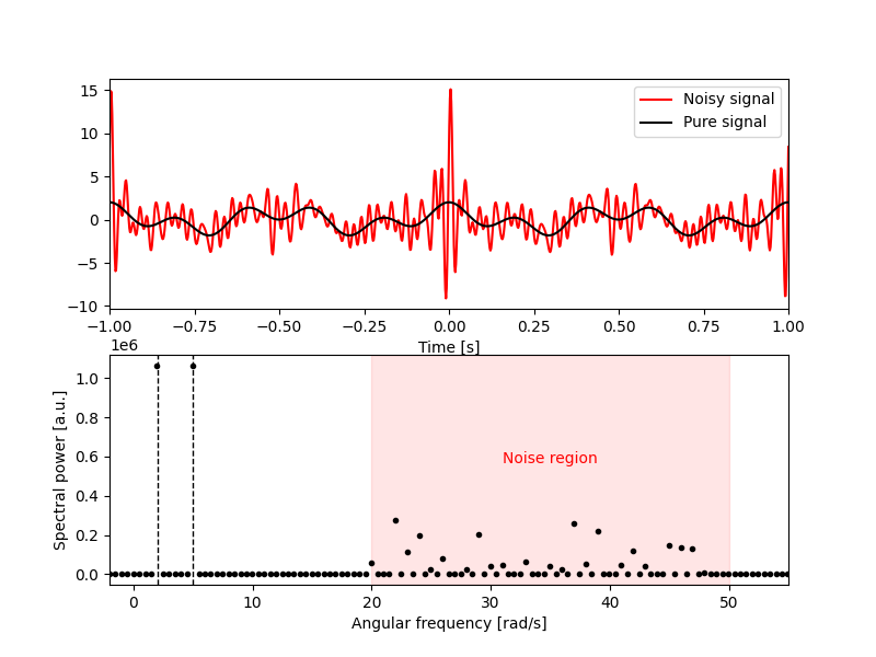
The basics of filtering is as follows: set the transform of a signal to 0 in regions which are thought to be undesirable. In the case of the Fourier transform, this is known as a band-pass filter; frequency components of a particular frequency band are passed-through unchanged, and frequency components outside of this band are zeroed. Special names are given to band-pass filters with no lower bound (low-pass filter) and no upper bound (high-pass filter). We can express this filtering as a window function $W_k$ in the inverse discrete Fourier transform:

$$x_{n}^{\text{filtered}} = \frac{1}{N}\sum_k W_k \cdot X_k \cdot e^{i 2 \pi k n / N}$$

In the case of the plot above, we want to apply a low-pass filter with a cutoff at $\omega=10$. That is:

$$W_k = \left\{ \begin{array}{cl} 1 & : \ |k| \leq 10 \\ 0 & : \ |k| > 10 \end{array} \right.$$

Visually:

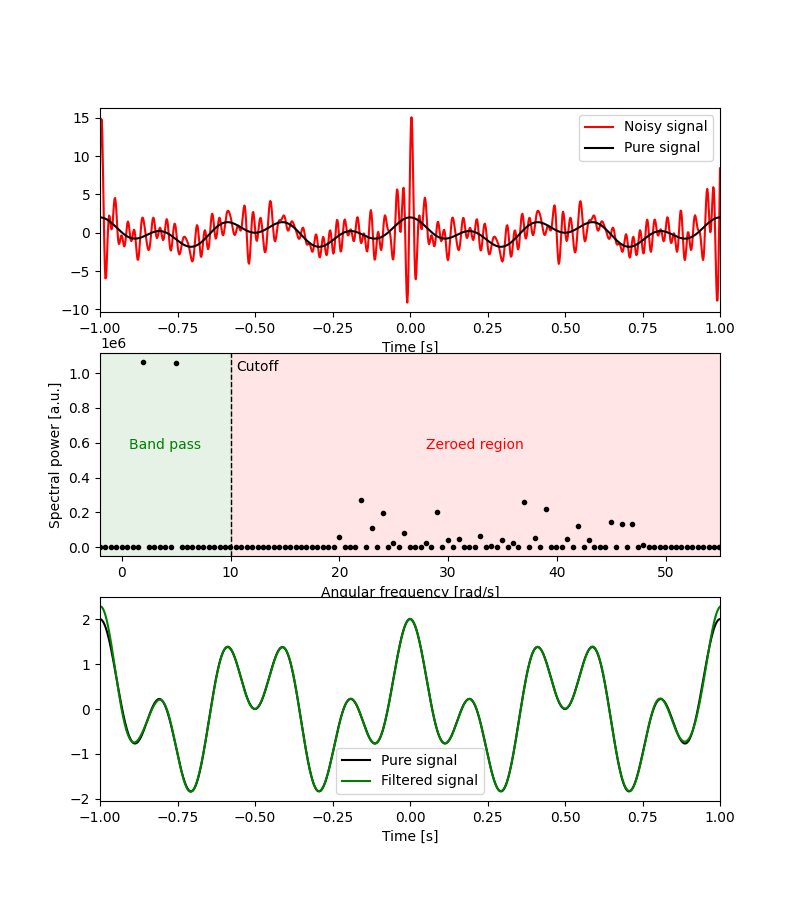
The lesson here is that filtering signals using a discretized integral transform (like the discrete Fourier transform) consists in:

1. Performing a forward transform;
2. Modifying the transformed signal using a window function, usually by zeroing components;
3. Performing the inverse transform on the modified signal.

Discrete wavelet transforms

Discrete wavelet transforms are a class of discrete transforms which decomposes signals into a sum of wavelets. While the complex exponential functions which make up the Fourier transform are localized in frequency but infinite in space, wavelets are localized in both time space and frequency space.

In order to generate the basis wavelets, the original wavelet is stretched. This is akin to the Fourier transform, where the sine/cosine basis functions are ‘stretched’ by decreasing their frequency. In technical terms, the amount of ‘stretch’ is called the level. For example, the discrete wavelet transform using the db4⁴ wavelet up to level 5 is the decomposition of a signal into the following wavelets:

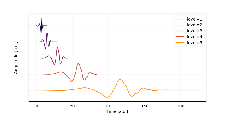
In practice, discrete wavelet transforms are expressed as two transforms per level. This means that a discrete wavelet transform of level 1 gives back two sets of coefficients. One set of coefficient contains the low-frequency components of the signal, and are usually called the approximate coefficients. The other set of coefficients contains the high-frequency components of the signal, and are usually called the detail coefficients. A wavelet transform of level 2 is done by taking the approximate coefficients of level 1, and transforming them using a stretched wavelet into two sets of coefficients: the approximate coefficients of level 2, and the detail coefficients of level 2. Therefore, a signal transformed using a wavelet transform of level $N$ has $N$ sets of coefficients: the approximate and detail coefficients of level $N$, and the detail coefficients of levels $N-1$, $N-2$, …, $1$.

Filtering using the discrete wavelet transform

The discrete Fourier transform excels at filtering away noise which has nice properties in frequency space. This is isn’t always the case in practice; for example, noise may have frequency components which overlap with the signal we’re looking for. This was the case in my research on ultrafast electron diffraction of polycrystalline samples^{5 6}, where the ‘noise’ was a trendline which moved over time, and whose frequency components overlapped with diffraction pattern we were trying to isolate.

As an example, let’s use real diffraction data and we’ll pretend this is a time signal, to keep the units familiar. We’ll take a look at some really annoying noise: normally-distributed white noise drawn from this distribution⁷:

$$P(x) = \frac{1}{\sqrt{2 \pi}} \exp{-\frac{(x + 1/2)^2}{2}}$$

Visually:

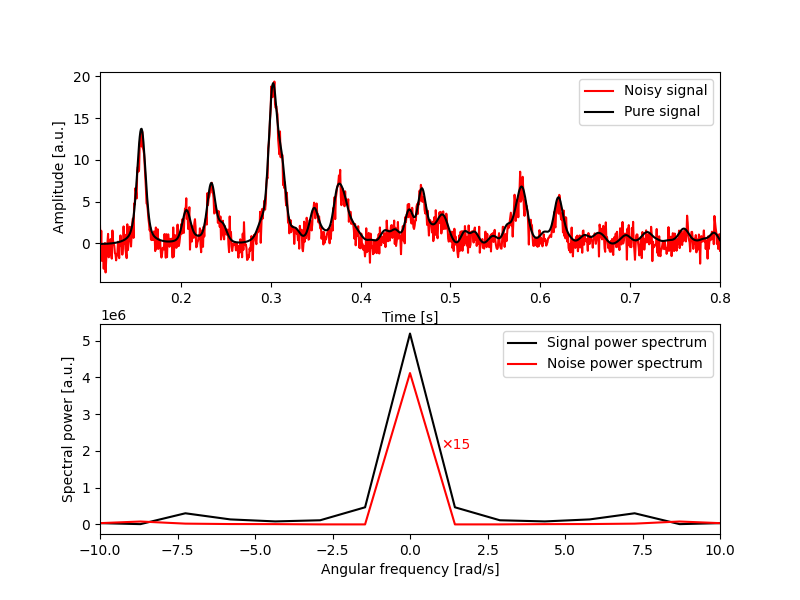
This example shows a common situation: realistic noise whose frequency components overlap with the signal we’re trying to isolate. We wouldn’t be able to use filtering techniques based on the Fourier transform.

Now let’s look at a particular discrete wavelet transform, with the underlying wavelet sym17. Decomposing the noisy signal up to level 3, we get four components:

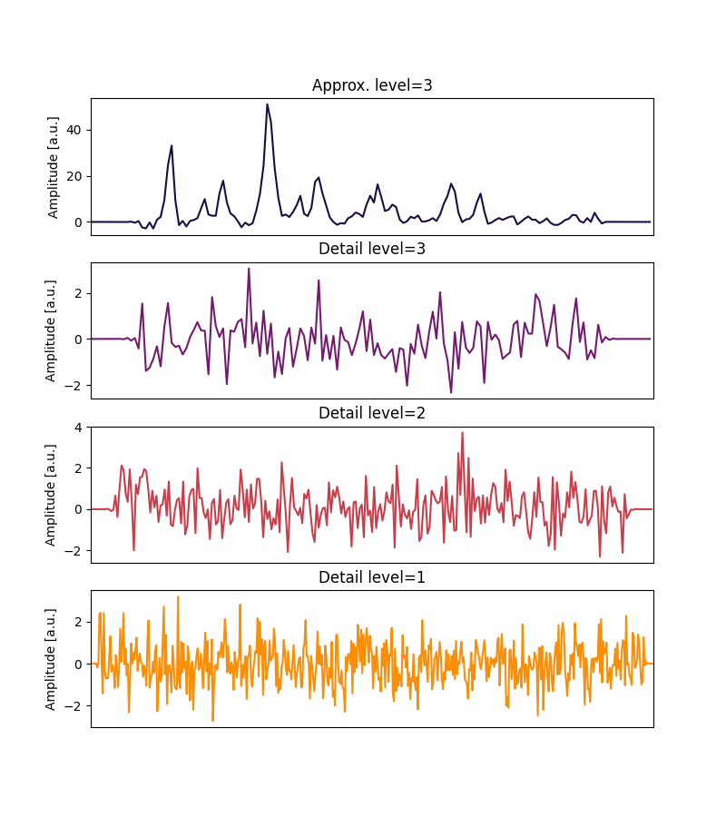
Looks like the approximate coefficients at level 3 contain all the information we’re looking for. Let’s set all detail coefficients to 0, and invert the transform:

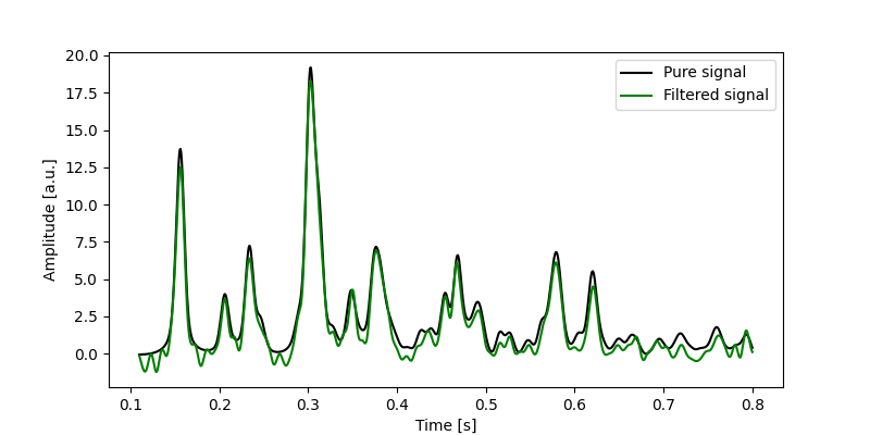
That’s looking pretty good! Not perfect of course, which I expected because we’re using real data here.

Conclusion

In this post, I’ve tried to give some of the intuition behind filtering signals using discrete wavelet transforms as an analogy to filtering with the discrete Fourier transform.

This was only a basic explanation. There is so much more to wavelet transforms. There are many classes of wavelets with different properties, some of which⁸ are very useful when dealing with higher-dimensional data (e.g. images and videos). If you’re dealing with noisy data, it won’t hurt to try and see if wavelets will help you understand it!