Exploring the multiverse of possibilities all at once using monads

I’m working on a global optimization problem these days. Unlike local optimization problems, e.g. what you would solve using least-square minimization, global optimization inevitably involves exhaustively evaluating all possible solutions and choosing the best one. As you can imagine, global optimization is much more computationally-intensive than local optimization, due to the size of the set of potential solutions. Speeding up a global optimization problem involves reducing the set of possible solution to a minimum, based on the specifics of the problem.

In this post, I’ll show you how to build the minimal set of possible solutions to an optimization problem, instead of searching for solutions in a larger space. As we’ll see, only viable solutions are ever considered. This will be done by splitting the computations into multiple universes whenever a choice is presented to us, such that we traverse the multiverse of possibilities all at once.

An example problem

Let’s say we’ve got 8 friends going out for a drink, in two cars with four seats each. How many arrangements of people can we have? If we don’t care about where people sit in each car, the number of arrangements is the number of combinations of 4 people we can make from 8 people, since the remaining 4 people will go in the second car. For every configuration, there’s also a configuration which swaps the car. Therefore, there are:

$$\binom{8}{4} \times 2 = \frac{8!}{4!(8-4)!} \times 2 = 140$$

possible combinations. If you’re not familiar with this notation, you can read $\binom{8}{4}$ as choose 4 people out of 8 people, of which there are 70 possibilities (and then 70 other possibilities with the cars swapped). That means that if we wanted to optimize the distribution of people into the two cars – for example, if we wanted to group up the best friends together, or minimize the total weight of people in car1, or some other objective –, we would need to look at 140 solutions. This problem is purely combinatorial.

Now let’s add some constraints. Our 8 friends are coming back from the bar. Out of the 8 friends, 3 of them didn’t drink and are therefore allowed to drive. Thus, the number of possible arrangements of friends in the car has been reduced, as each car needs a driver. For one car, we need to select 1 driver out of 3, and 3 remaining passengers out of 7. However, the other car will need a driver, so really there are 6 passengers to choose from. Finally, for every arrangement there is a duplicate arrangement with the cars swapped. The number of possibilities is therefore:

$$\binom{3}{1} \binom{6}{3} \times 2 = 120$$

Potential solutions as a decision graph

How else can we express the number of combinations? Think of building a solution, instead of searching for one. We may want to start by assigning a driver to car 1. For each possible decision here, we’ll assign a driver to the second car next, then passengers. The possibilities look like this:

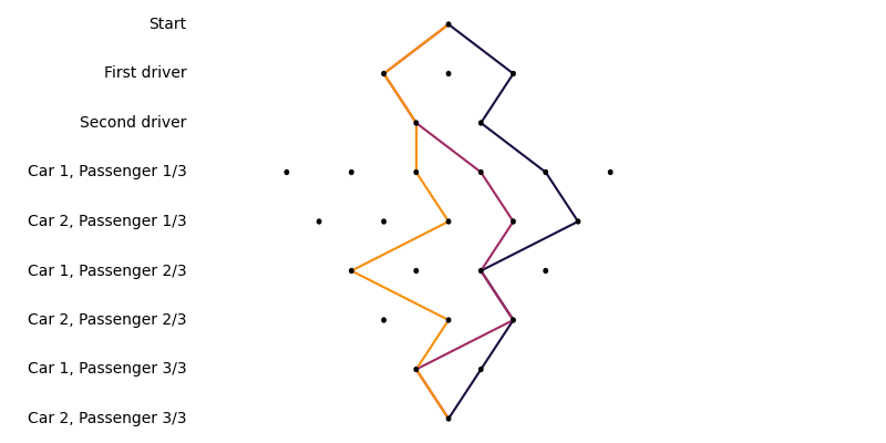
In the figure above, no one is assigned at the start. Then, we assign the first driver (out of three choices). Then, we need to assign a second driver, of which there are only two remaining. Each of the 6 passengers are then assigned. A potential solution (i.e. a assignment between people and cars) is represented by a path in the decision tree. Three possibilities are shown as examples.

This way of thinking about solutions reminds me strongly of the Everett interpretation of quantum mechanics, also known as the many-worlds interpretation or the multiverse interpretation. The three potential assignments are three universes that split from the same starting point. Enumerating all possible solutions to our example problem consists in crawling the decision tree, or crawling the multiverse of possibilities.

Expressing the multiverse of solutions in Haskell

Based on the decision tree above, I want to run a computation which, when presented with choices, explores all possibilities all at once.

Consider the following type constructor:

newtype Possibilities a = Possibilities [a]

A computation that returns a result Possibilities a represents all possible answers of final type a. For example, a computation can possibly have multiple answers might look like:

possibly :: [a] -> Possibilities a
possibly xs = Possibilities xs

Alternatively, a computation which is certain, i.e. has a single possibility, is represented by:

certainly :: a -> Possibilities a
certainly x = Possibilities [x] -- A single possibility = a certainty.

Possibilities is basically a list, so we’ll start with a Foldable instance which is useful for counting the number of possibilities using length:

instance Foldable Possibilities where
    foldMap m (Possibilities xs) = foldMap m xs

Possibilities is a functor:

instance Functor Possibilities where
    fmap f (Possibilities ps) = Possibilities (fmap f ps)

The interesting tidbit starts with the Applicative instance. Combining possibilities should be combinatorial, e.g. combining the possibilities of 3 drivers and 6 passengers results in 18 possibilities.

instance Applicative Possibilities where
    pure x = certainly x -- see above

    (Possibilities fs) <*> (Possibilities ps) = Possibilities [f p | f <- fs, p <- ps]

Recall that the list comprehension notation is combinatorial, i.e. [(n,m) | n <- [1..3], m <- [1..3]] has 9 elements ([(1,1),(1,2),(1,3),(2,1),(2,2),(2,3),(3,1),(3,2),(3,3)]).

Now for the crucial part of composing possibilities. We want past possibilities to influence future possibilities; we’ll need a monad instance. A monad instance means that if we start with multiple possibilities, and each possibility can results in multiple possibilities, the whole computation should produce multiple possibilities¹.

instance Monad Possibilities where

    Possibilities ps >>= f = Possibilities $ concat [toList (f p) | p <- ps] -- concat :: [ [a] ] -> [a]
        where
            toList (Possibilities xs) = xs

Let’s define some helper datatypes and functions. We

{- 
With the following imports:

import           Data.Set    (Set, (\\))
import qualified Data.Set as Set 
-}

-- | All possible people which can be assigned to cars
data People = Driver1    | Driver2    | Driver3
            | Passenger1 | Passenger2 | Passenger3
            | Passenger4 | Passenger5 | Passenger6
    deriving (Bounded, Eq, Enum)


-- A car assignment consists in two cars, each with a driver, 
-- as well as passengers
data CarAssignment 
    = CarAssignment { driver1        :: Person
                    , driver2        :: Person
                    , car1Passengers :: Set Person
                    , car2Passengers :: Set Person
                    }
    deriving Show


allDrivers :: Set Person
allDrivers = Set.fromList [Driver1, Driver2, Driver3]


-- Pick a driver from an available group of people.
-- Returns the assigned driver, and the remaining unassigned people
assignDriver :: Set Person -> Possibilities (Person, Set Person)
assignDriver people 
    = possibly [ (driver, Set.delete driver people) 
               | driver <- Set.toList $ people `Set.intersection` allDrivers
               ]


-- Pick three passengers from an available group of people.
-- Returns the assigned passengers, and the remaining unassigned people
assign3Passengers :: Set Person -> Possibilities (Set Person, Set Person)
assign3Passengers people = possibly [ (passengers, people \\ passengers) 
                                   | passengers <- setsOf3
                                   ]
    where setsOf3 = filter (\s -> length s == 3) $ Set.toList $ Set.powerSet people

Finally, we can express the multiverse of possible drivers-and-passengers assignments with great elegance. Behold:

carAssignments :: Possibilities CarAssignment
carAssignments = do
    let everyone = Set.fromList $ enumFromTo minBound maxBound -- [Driver1, Driver2, ..., Passenger6]
    
    (driver1, rest) <- assignDriver everyone
    (driver2, rest) <- assignDriver rest

    (car1Passengers, rest) <- assign3Passengers rest
    (car2Passengers, _)    <- assign3Passengers rest

    return $ CarAssignment driver1 driver2 car1Passengers car2Passengers

Given the monad instance for Possibilities, the return function returns all possible possibilities. Let’s take a look at the size of the multiverse in this case:

ghci> let multiverse = carAssignments
ghci> print $ length multiverse
120

Just as we had calculated by hand. Amazing!

Conclusion

What I’ve shown you today is how to structure computations in such a way that you are exploring the multiverse of possibilities all at once. The seasoned Haskell programmer will have recognized that the Functor, Applicative, and Monad instances of Possibilities are just like lists!

Although I’m not using Haskell at work², I expect that something similar will need to be built in the near future to speed up our global optimization problem. The specific problem we are tackling has many more constraints than the example presented in this post. It’s easier to generate a list of solutions, most of which are unsuitable, and filter the solutions one by one. There is a fixed computational cost associated with generating and checking a solution, and so reducing the set of possible solutions is even more important.

This post was partly inspired by the legendary blog post Typing the technical interview

A self-contained Haskell source file containing all code from this post is available for download here